## Excel visualization walk-through ### Cooper Comics Collection data - We will use the **Cooper Comics Collection** dataset. - In this example, we will work in the **Cooper Collection Books** sheet. - The same process can be adapted to a different sheet, field, or question. [Cooper Comics Collection data](https://mikrowelle.github.io/cooper-comics-final/data/Cooper%20Comics%20Reprint%20Metadata.xlsx)
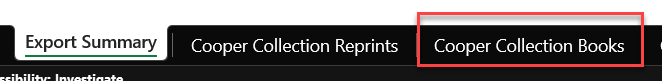
## 1. Open the dataset - Open the Excel file. - We will work in the **Cooper Collection Books** sheet.
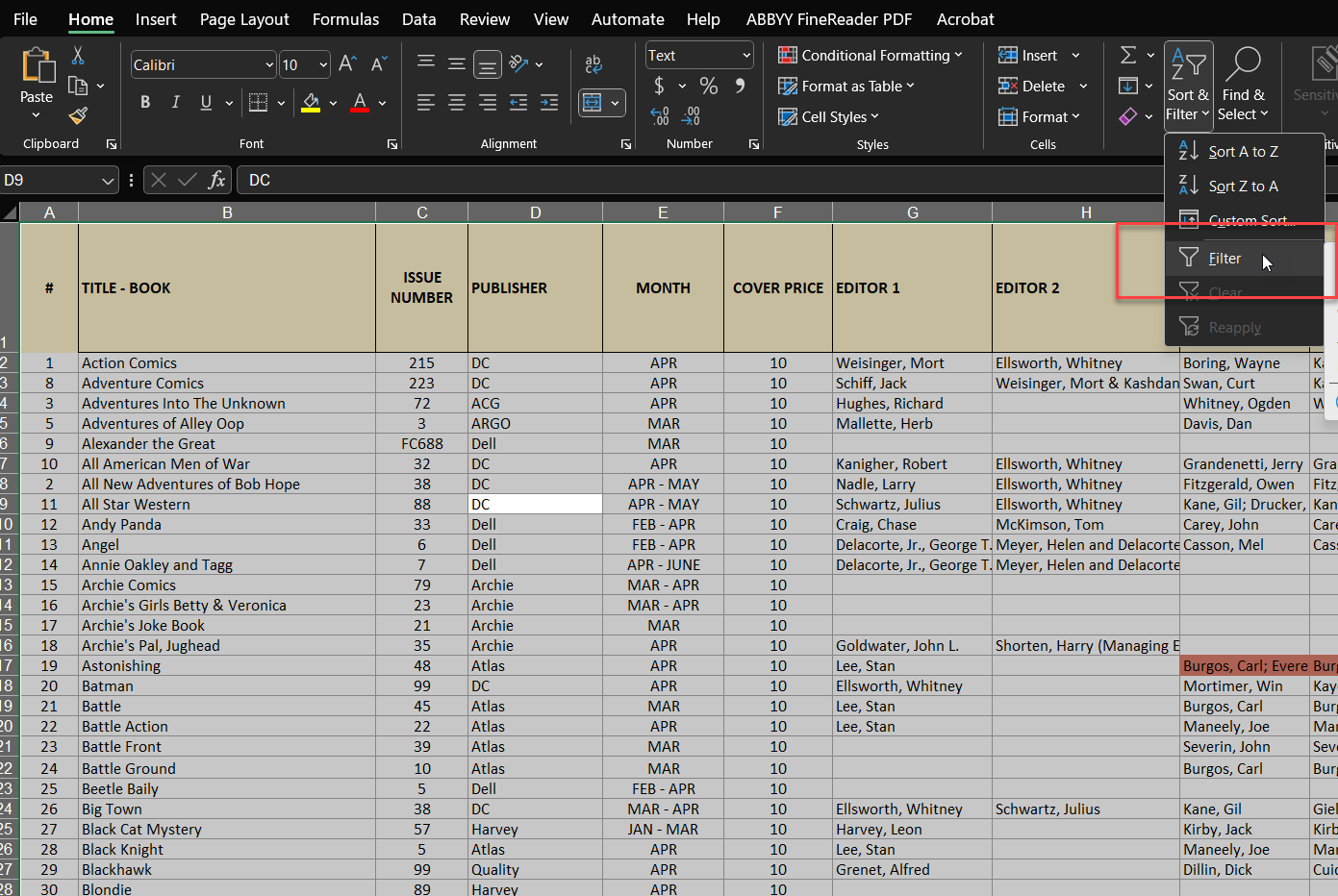
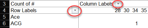
## 2. Turn on filtering - Select the data in the sheet. - Go to **Home > Sort & Filter > Filter**. - Excel adds a dropdown arrow to each column header.
 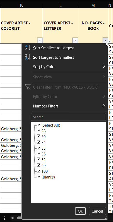
## 3. Example: filter by page count To show only books with **36 pages**: 1. Open the filter for **No. Pages - Book** 2. Clear **Select All** 3. Select **36** 4. Click **OK**
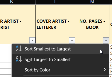
## 4. Sorting You can also sort values with the same dropdown menus. - number columns: **Smallest to Largest** or **Largest to Smallest** - text columns: **A to Z** or **Z to A**
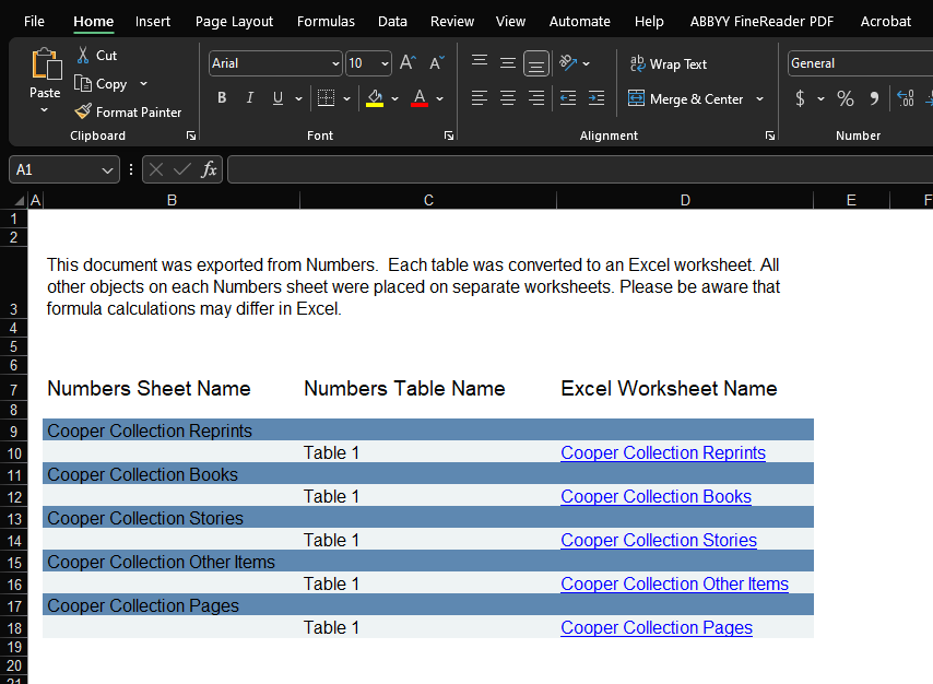
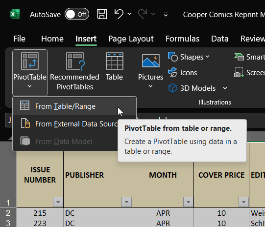
## 5. Create a pivot table - Select the data in **Cooper Collection Books** - Go to **Insert > PivotTable** - Keep the selected range - Leave **New Worksheet** selected - Click **OK** Note: > A PivotTable is a tool for summarizing raw spreadsheet data. Instead > of looking at one row at a time, you can group records by category > and count, total, or compare them. A regular table stores the > original data; a PivotTable helps you see patterns in that data. > It is useful for questions like: How many books belong to each > publisher or genre? >
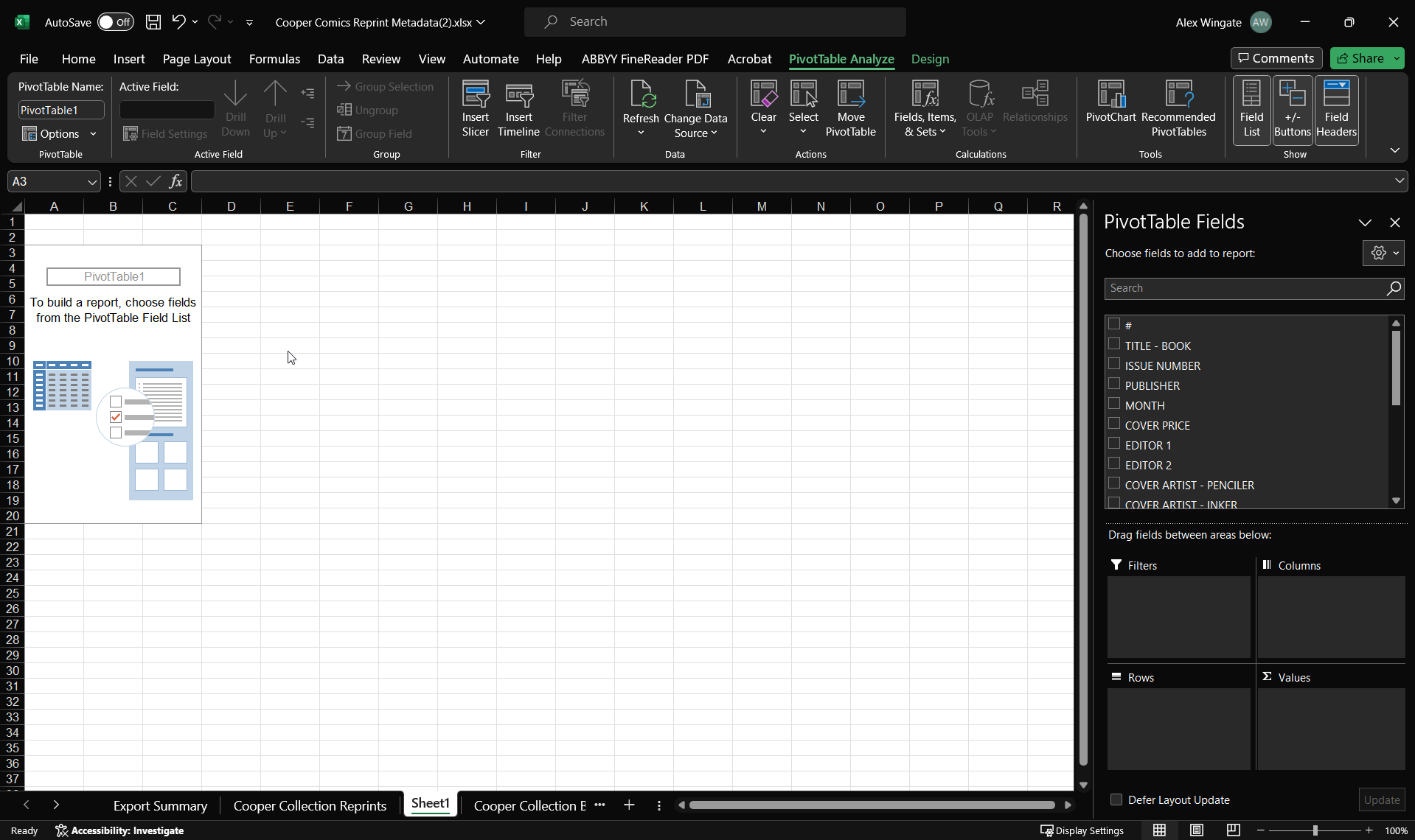
## 5. Create a pivot table Excel creates: - a new worksheet - an empty pivot table - a **PivotTable Fields** panel
 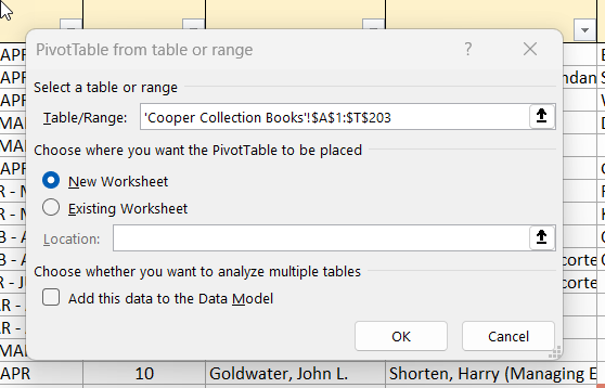 
 Creating new PivotTable worksheet
 PivotTable Fields panel
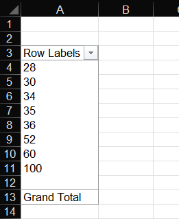
## 6. Count books by page length - Drag **No. Pages - Book** to **Rows** - Drag **#** to **Values** This sets up a pivot table that can count books by page count.
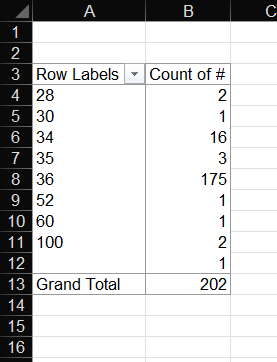
## 7. Change **Sum** to **Count** Excel may default to **Sum of #**. We want a **count**, not a sum. 1. Click **Sum of #** 2. Choose **Value Field Settings** 3. Select **Count** 4. Click **OK** <aside class="notes"> <p>You should now see the number of books for each page length. </p> <p> This is the main conceptual move. Students are aggregating the data instead of reading row by row.</p> </aside>
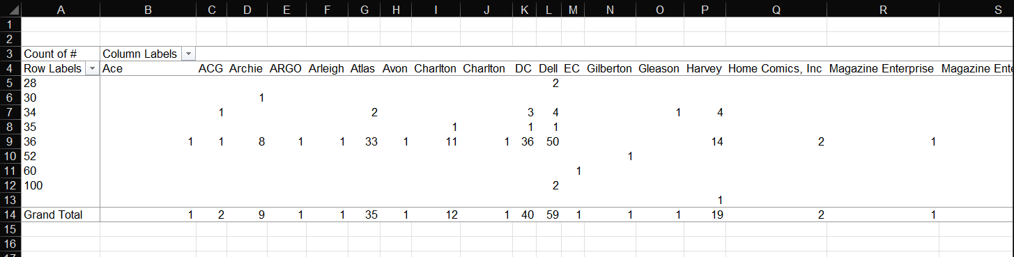
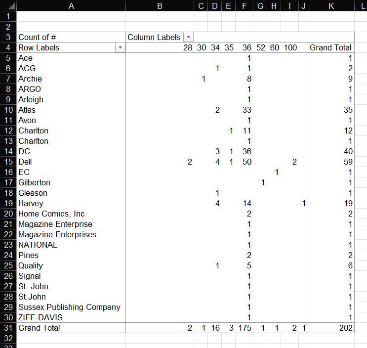
## 8. Add another variable You can compare page count with another category. Example: - drag **Publisher** to **Columns** This shows the count of books for each combination of: - **page count** - **publisher**
## 8. Add another variable If the table is hard to read: - move **Publisher** to **Rows** - move **No. Pages - Book** to **Columns** This layout is often easier to scan.
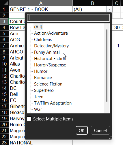
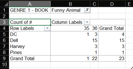
## 9. Filter the pivot table You can also filter the pivot table itself. Example: - drag **Genre 1 - Book** to **Filters** - choose a value such as **Funny Animal**
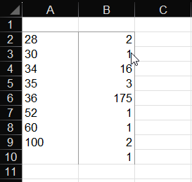
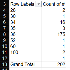
## 10. Prepare to chart the pivot table Set up the pivot table so that: - **No. Pages - Book** is in **Rows** - **Count of #** is in **Values** Then copy the page-count and count values into a new worksheet.
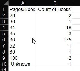
## 10. Prepare to chart the pivot table In the new worksheet: - add clear column headings - if one row has no page-count value, label it **Unknown**
## 11. Choose a chart type A **bar chart** or **column chart** works well here because you are comparing category counts. - Select the copied data - Go to **Insert > Charts** - Choose a **bar chart** or **column chart**
<!-- ## 11. Choose a chart type Excel inserts the chart into the worksheet. This gives you a first draft of the visualization.--> 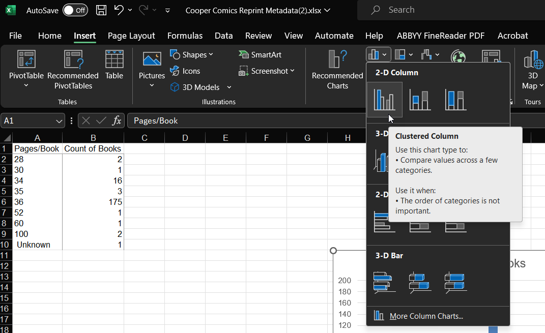
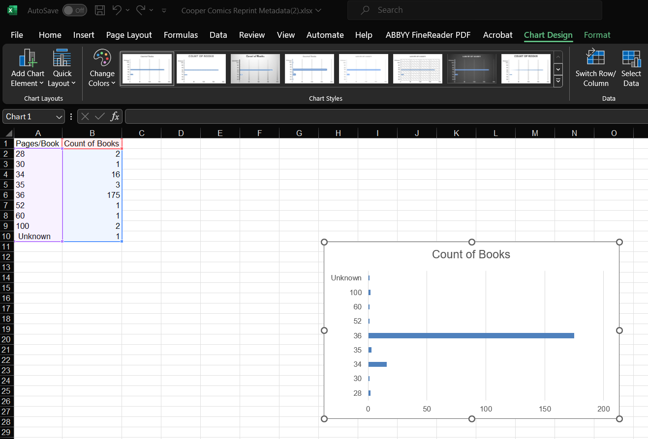
## 12. Improve readability With the chart selected: - edit the chart title - add axis titles - check whether the labels are readable - adjust spacing, font size, or axis settings if needed
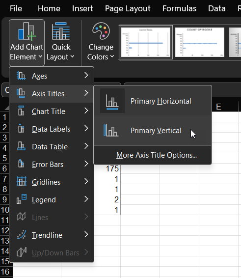
## 12. Improve readability Use: - **Chart Design > Add Chart Element > Axis Titles** - double-click the title to edit it - the formatting sidebar for additional changes Do not get stuck polishing.
 <aside class="notes"> Instructor note: Do not let students get stuck polishing. Clear title, readable labels, and a sensible chart type are enough. </aside>
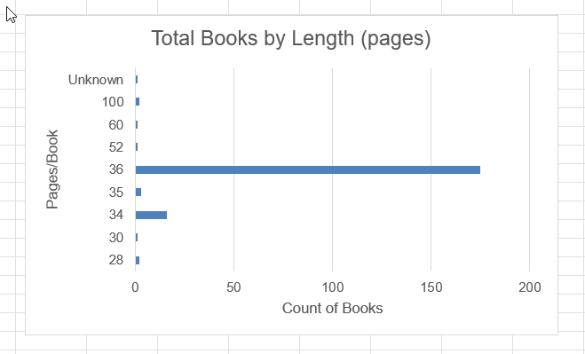 _Edit chart title._ --- 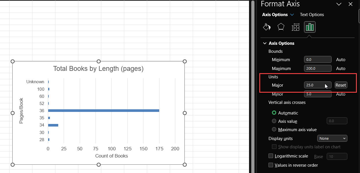 _Format axis options._ --- 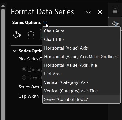 _Format sidebar._
## By the end, you should have - one filtered view of the data - one pivot table - one chart based on that pivot table The goal is not a perfect chart. The goal is to move from spreadsheet data to a simple, readable visualization.